Try the math for yourself (requires Maple)
Illustration of the Romney Tax Plan
(In which we learn that the math adds up, but the real world assumptions may not)
| > |
 |
We will approximate household income as being gamma distributed.
We are able to match our CDFs to available data points quite closely.
| > |
 |
Approximate all households of a particular income pay the same (2012) taxrate (ignore marital status, etc).
| > |
![incomebrackets := Vector([0, 10500, 18500, 22500, 30000, 35000, 55000, 62500, 77500, 92000, 167000, 250000, 350000], datatype = float); -1](images/romney_tax_plan_3.gif)
![incomebrackets := Vector([0, 10500, 18500, 22500, 30000, 35000, 55000, 62500, 77500, 92000, 167000, 250000, 350000], datatype = float); -1](images/romney_tax_plan_4.gif) |
| > |
![tb := [0, 17400, 70700, 142700, 217450, 388350, 1000000]; -1](images/romney_tax_plan_5.gif) |
Feed in 2006 data for US, and a simulated Romney-world where income tax has been cut across the board by 20%
| > |
![incomeupperpercentiles := Vector([0, .1, .2, .25, .33, .4, .6, .67, .75, .8, .95, .985, .99], datatype = float); -1](images/romney_tax_plan_6.gif)
![incomeupperpercentiles := Vector([0, .1, .2, .25, .33, .4, .6, .67, .75, .8, .95, .985, .99], datatype = float); -1](images/romney_tax_plan_7.gif) |
| > |

 |
| > |
 |
| > |
 |
| > |
 |
| > |
![Fit(gammacdf(i, k, theta), incomebrackets, incomeupperpercentiles, i, output = parametervalues, initialvalues = [k = 2, theta = 22000])](images/romney_tax_plan_13.gif)
![Fit(gammacdf(i, k, theta), incomebrackets, incomeupperpercentiles, i, output = parametervalues, initialvalues = [k = 2, theta = 22000])](images/romney_tax_plan_14.gif) |
![[k = HFloat(1.4412610258235732), theta = HFloat(39576.22398588795)]](images/romney_tax_plan_15.gif) |
(1) |
Here are curves to match some real world data (2006)
| > |

 |
Here are some example curves that would increase revenue while cutting taxes 20% across the board
This is the fishy part of Romney's plan. He's offered no numbers to support the claim that his plan
for the economy would produce anything like this.
| > |
 |
| > |
 |
| > |
 |
| > |

 |
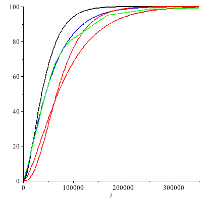
Plotting %US Households < particular household income
Black line is the "best guess" we fed into the curve fitter.
Blue is the output distribution that is the result of a least squares
regression to the gamma CDF. Green is real world data.
Red lines are possible "Romney-world CDFs"
| > |
![display([guess, fitplot, romplot, rom2plot, dataplot])](images/romney_tax_plan_23.gif) |
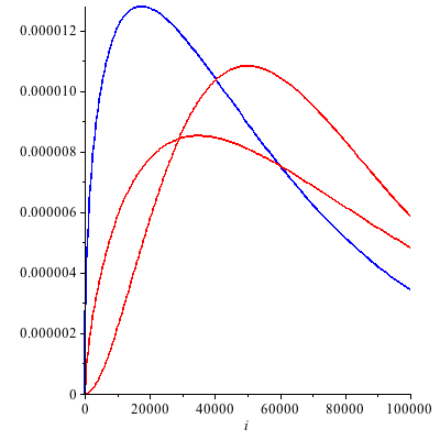
Distribution function showing modal income.
Normalized so that the total area under the curve
represents the number of households (i.e., area scaled by 1/110000000)
| > |
 |
| > |
 |
| > |
 |
| > |
![display([curpdfplot, rompdfplot, rom2pdfplot])](images/romney_tax_plan_28.gif) |
And some income-tax revenue calculations based on our approximated real world
compared with 2 possible Romney worlds.
| > |
 |
 |
(2) |
| > |
 |
 |
(3) |
| > |
 |
 |
(4) |
Conclusions: It IS possible to cut taxes across the board while increasing revenue.
The real question is whether or not the economic assumptions required to do so are valid.
I do not have any data on this point. So the question is, do you believe Romney's election
can effect the economy this drastically?
For a much simpler and more assured path to a balanced budget,
check out Libertarian Presidential Candidate Gary Johnson.


